Difference Method
(1) Difference Method, Advantages
(2) Differential Method and Difference Method
(2)-1 Comparison between Differential and Difference Methods
(2)-2 Error of Forward Difference
(2)-3 Expression of First-Order Differentiation in Difference
(2)-4 Expression of Second-Order Differentiation in Difference
(3) Calculation of Difference in Excel
(3)-1 Calculated Spreadsheet
(3)-2 3D
(1) Difference Method, Advantages
The differential equations can be expressed with no error when we expand it to an infinite series. However, it is impossible to calculate the infinite series, and therefore, we use the finite numbers out of the infinite one. It automatically generates the error. For example, if the first two (2) items, the third and later ones are the error. Once the error is small enough for the calculation purpose, the finite series becomes the solution of the differential equation. The biggest advantage of the difference method is that we can see the further state change of the differential equation, which has no analytical solution. It means that we can practically simulate the phenomena if we can minimize the error.
Specifically, the difference method is an approximate solution method of differential equations. It is the Taylor expansion of the differential equations. If we know the spatial distribution at time is zero (0), we can calculate the new distribution after a very short time. It can be continued one after another. (It is an explicit method.) Unlike the finite element method, we can get the solution even if we do not have the approximate formula, which are obtained from the specialized knowledge of the phenomena.
(2) Differential Method and Difference Method
Our great predecessors have been studying the differential equations. We can fully utilize their outcome. I would like to explain how to utilize those to the simulation.
The following picture shows a simple illustration of a heating furnace, where a hot area is seen on the top of the furnace. The material of the lower temperature enters into the furnace and moves to the right. During the movement, the temperature of the material becomes higher.
As an example, let's assume that we want to know the temperature of the center of a material in a heating furnace. The furnace is made of heat insulating material and the heating plate is set on the top of the furnace. The temperature distribution of the heating plate and the movement speed of the material is know.
For the case, we need to calculate the temperature of whole area of the heat insulating material as well as the material. It sounds simple, but the actual calculation is somehow complicated. Because there are many items to consider. For example, regarding the heat radiation, there are many sauces, one is from the plate, another from the walls, the third one from/to the both sides of the material. Then, the hotter air around the material convey the heat due to the air movement. Even if there is no intentional movement of air, the cold material in the hot air generate the natural air movement around the material. These are the input to the material. Once the heat is conveyed to the surface of the material, it moved into the material to reach the center.
We are going to calculate the temperature distribution of a round steel billet in a heating furnace. The applicable differential equation consists of the first- and second-order differential equations of heat energy. Please see the "Thermodynamics" for detail. Here in the numerical analysis, it is similar to the equations of motion of the bodies.
The equation of motion of the bodies indicates the force F is equal to the mass m times acceleration a. F = ma. The first-order of position of the body is the velocity (speed), and second-order is the acceleration.
(2)-1 Comparison between Differential and Difference Methods
Let's see the comparison between the differential and the difference methods of one-dimension (1D), because it is easier to understand. The way of comparison of the two-dimensional (2D) and three-dimensional (3D) ones are same as the 1D.
The delta x of the differential method becomes as close as zero (0) and therefore there is no error. However, not all the differential equation can be solved.
The delta x of the difference method remains and therefore the error does exist. However, as seen in the illustration, when it is small enough, the error also reduced to fit the purpose of the analysis. In the actual engineering, there are errors in the measuring and deviations of the material dimensions and so on. Therefore, there should be the tolerable error in the solutions as well. The important thing is that we can get the solution even when there is no analytical solution to the original differential equation. We can make a program or utilize the spreadsheet for the solution.
The delta x is called the discretization. It is to divide the space or time to the finite numbers.
(2)-2 Error of Forward Difference
The fx is the measured number and the fx+1 is the unknown one. The word "forward" means the next one. The opposite side is the "backward" and the backward difference can be defined as well; however, the "forward" one is enough and let's forget the "backward" one.
The delta x of the differential method becomes as close as to zero (0) and therefore it does not contain an error. Therefore, the differential equations give the analytical solutions with no error as long as we can solve them; however, many of them cannot be solved. On the contrary, the difference method gives the next value fx+1 with an error. Therefore, the difference equations always give the solutions. It is necessary to evaluate and to minimize the error.
The Taylor expansion is used for the calculation of the fx+1. The Taylor expansion calculates the next value fx+1 by the known fx times and the slope times the distance delta x. However, the multiplication is not enough. In order to make up the gap, the further correction continue infinitely. The following formula shows the definition of the Taylor expansion.
The important thing of the error is that the error is calculated as the delta x times something. It means, the smaller delta x, the smaller error. The above graphic indicates the smaller delta x can reduce the error, and the definition of the Taylor expansion clearly proves it.
(2)-3 Expression of First-Order Differentiation in Difference
The Taylor expansion is the finite series, which is impossible to calculate. In my humble opinion, the laptops can help the calculation up to any order you prefer; however, if we follow the historical one, we use the series up to the second order, and the third and higher are the error. If it is so, we can use the spreadsheet as well as the programming for the calculation.
Fist of all, let's consider the first-order of the Taylor expansion. The following piecure shows the three (3) kinds of the difference.
There is no rule which of the three (3) to use. However, the central difference is suggested. The formula of the central difference is also shown in the above picture.
(2)-4 Expression of Second-Order Differentiation in Difference
The first-order differential formula is the slope and the second-order one is the slope of the slope. The second-order central difference is defined as the slope between the first-order forward difference and first-order backward difference. (Please let me skip the rest of the expression.)
(3) Simulation by the Difference Method
Both of the first- and second-order of the difference equations are obtained. The simulation by the difference method is very simple. It is just replace the differential equation by the difference ones. The differential equation will be easily converted to the fx+1= type of equation.
Let's assume that the differential equation of a material is defined as the function of the time and the positions. For example, the thermal conduction equation can be simplified as the change by time is proportional to the second-order of the positions. Please find the calculation sequence as follows.
(1) Convert the differential equation to the difference one.
(2) Descrive the initial condition before the calculation, which is time = zero (0).
(3) Repeat the calculation step by step, which is delta t.
(4) Output.
Thin and long bar or wire is considered as 1D. The cross section is considered as the 2D. The whole area of a body is 3D.
The outcome is a distribution of temperature, for example. It may be easy to understand the distribution if you draw the 3D graph.
(3) Calculation of Difference in Excel
(3)-1 Calculated Spreadsheet
The length of the formula is short enough for a cell of the spreadsheet when the calculation is limited up to the second-order ones. The maximum numbers of the letter in an Excel cell is about 32000. It can accept longer texts; however, shorter one is convenient for many reasons, such as finding typo.
It is necessary to pay attention to the boundary of the calculation area. we have selected the central deffirence; howver, the boundary is the rim and therefore either forward or backward difference is applicable to the rim.
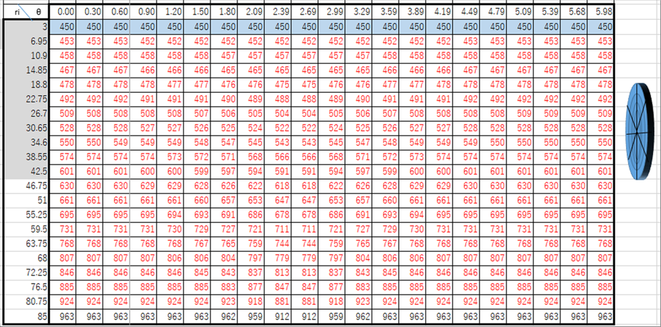
The following table shows the spreadsheet for the calculation of a round steel billet. The cylindrical coordination system is adopted for the round billet. The detail calculation is shown in the article "Temperature Calculation".
(3)-2 3D
The coordinate conversion from the cylindrical one to the spherical one gives the 3D view. It is possible to rotate along 3 axis. It looks easy to see the results.
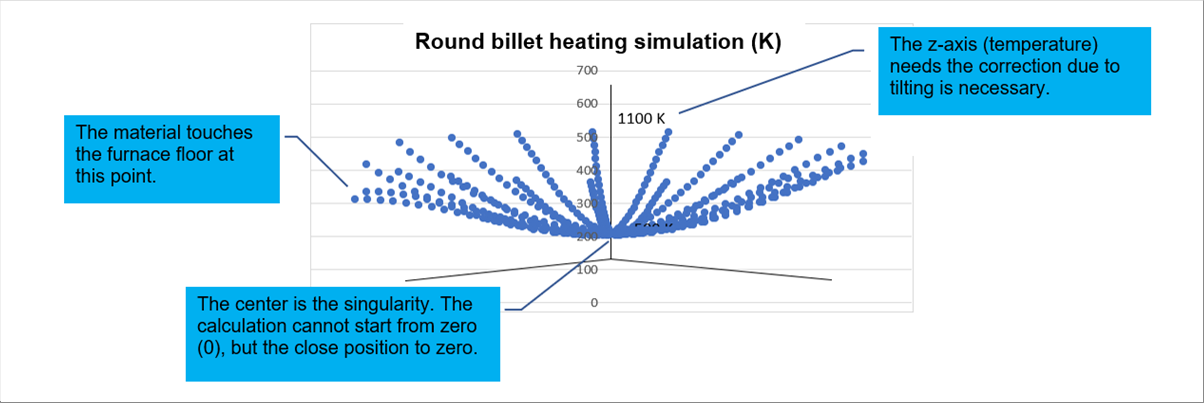
The following graph shows an example of the 3D view of the above spreadsheet. Please see the "3D View" for the detail calculation.
Please let me explain bit more for the comments in the 3D graph.
The center is a sigularity in the cylindrical coordination system. Therefore, the calculation starts from three (3) mm apart from the center to the outside of the billet.
The temperature of the floor where the round billet is heated is assumed is lower than that of the surrounded hot air. The material of the floor is assumed a heat insulating one, and the heat conductivity of the floor is different from the steel billet.
The vertical axis shows the converted one, which is different from the original one. It was because of the tilting of the axis. The typed 1100 K, shown between 500 and 600 on the vertical axis, is the converted value.
Author: T. Oda
The page was prepared in Excel, and automatic html and css generation by the "excel2web".